GenX-SE: Nordic 12-zone energy-system case

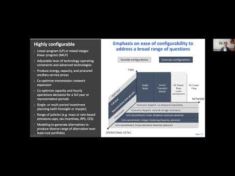
A GenX capacity-expansion + dispatch case covering all 12 Nordic bidding zones: Sweden (SE1–SE4), Norway (NO1–NO5), Finland (FI), and Denmark (DK1, DK2). 17 transmission lines including the three Swedish snitt cuts (1/2/4), six NO internal lines, and seven SE↔neighbor interconnectors. The AC vs HVDC distinction is preserved in line names — relevant if you later add CapacityReserveMargin or reserve-sharing logic (reserves only flow within a synchronous area; see CLAUDE.md).

Status: runnable scaffold with synthetic 8760-h profiles calibrated to plausible Nordic totals (≈380 TWh, peak ≈65 GW across the area). Resource capacities reflect roughly 2024-actual fleet sizes. All time-series data is synthetic — replace with ENTSO-E observations via data/fetch_entsoe.py before reporting results.

Topology

Zone	Region	Sync area	Avg demand
SE1	Norrbotten (Luleå)	Nordic	2.0 GW
SE2	Mid-Norrland (Sundsvall)	Nordic	2.5 GW
SE3	Mälardalen / Stockholm	Nordic	8.5 GW
SE4	Skåne / South (Malmö)	Nordic	3.0 GW
NO1	Oslo / Eastern Norway	Nordic	4.1 GW
NO2	South Norway / Stavanger	Nordic	4.1 GW
NO3	Mid-Norway / Trondheim	Nordic	2.5 GW
NO4	Northern Norway / Tromsø	Nordic	1.8 GW
NO5	Western Norway / Bergen	Nordic	2.5 GW
FI	Finland	Nordic	9.1 GW
DK1	Jutland + Fyn	Continental	2.8 GW
DK2	Zealand (Copenhagen)	Nordic	1.4 GW

Transmission lines

Three groups of inter-zonal links (NTC values reflect minRAM-compliant market-available capacity):

SE internal snitt (AC): SE1↔SE2 3300, SE2↔SE3 7300, SE3↔SE4 5400

SE↔neighbor (mix of AC and HVDC):

• SE1↔NO4 Ofoten (AC) 700
• SE2↔NO3 Nea (AC) 1000
• SE3↔NO1 Hasle (AC) 2050
• SE1↔FI Tornehamn (AC) 1500
• SE3↔FI Fenno-Skan (HVDC) 1200
• SE3↔DK1 Konti-Skan (HVDC) 740
• SE4↔DK2 Öresund (AC) 1700

NO internal + NO↔DK (AC except Skagerrak):

• NO1↔NO2 3500, NO1↔NO3 500, NO1↔NO5 600
• NO2↔NO5 600, NO3↔NO4 600, NO3↔NO5 500
• NO2↔DK1 Skagerrak (HVDC) 1632

These values are NTC made available to the market (post-minRAM), not raw thermal line capacity. Under EU Regulation 2019/943 Article 16(8), TSOs must make at least 70% of the operationally secure cross-zonal capacity available for cross-zonal trade — internal grid congestion is not a valid reason to reduce it below that floor. The rule (often called minRAM, Minimum Remaining Available Margin) has been binding since 31 December 2025. Svenska Kraftnät has had documented compliance shortfalls during high-demand periods, especially on snitt 4 (SE3↔SE4) — N-1 contingencies in the SE3 grid drove the 2011 zonal split and remain the binding constraint. Energimarknadsinspektionen (Ei) is currently reviewing SvK's compliance after ACER flagged the issue. To model non-compliant operating modes or alternative trajectories, multiply these values by your assumed fraction (0.50 / 0.70 / 1.00) and re-run.

Generation fleet (existing capacities, MW)

Resource	SE1	SE2	SE3	SE4	NO1	NO2	NO3	NO4	NO5	FI	DK1	DK2
Hydro reservoir	5300	8200	2700	300	5000	10000	4000	6000	8000	3200	–	–
Nuclear	–	–	6900	–	–	–	–	–	–	4400	–	–
Biomass CHP	200	400	2000	800	–	–	–	–	–	2500	2500	1000
Gas / oil peaker	–	–	–	1700	–	700	–	–	–	–	200	–
Onshore wind	2400	5400	4500	1700	500	1500	2000	1000	200	6900	3400	700
Offshore wind	–	–	–	200	–	–	–	–	–	–	1700	400
Solar PV	–	–	1800	600	–	–	–	–	–	700	2000	1000
Battery storage	0	0	0	0	0	0	0	0	0	0	0	0

Existing nuclear, oil, gas, and hydro are no-new-build, can-retire so the model chooses whether to keep them economical. All renewables, batteries, and biomass CHP can expand. Hydro reservoirs are existing-only (limited expansion potential everywhere except possibly NO).

How to run

make install      # Julia + GenX + Python (uv) — first time only
make run-fast     # solve with TimeDomainReduction=1 (≈30s with HiGHS)
make plot         # PNG + interactive HTML in plots/output/
# or just:
make all

Detailed runbook: HOW_TO_RUN.md.

1-hour vs 15-minute resolution

The Nordic synchronous area moved to a 15-min Imbalance Settlement Period in 2023–2024, and the day-ahead market (Nord Pool / SDAC) went 15-min in October 2025. The case ships at 1-hour by default (8760 steps); switch to 15-min with:

make to-15min     # regenerate timeseries + rescale resource CSVs (8760 -> 35040)
make run          # full-resolution solve
make to-1h        # revert

scripts/rescale_resources.py is what makes this safe: it multiplies Up_Time / Down_Time / Min_Duration / Max_Duration by 4 and divides Ramp_Up_Percentage / Ramp_Dn_Percentage by 4 so the physical behaviour stays the same (e.g. a 6-hour minimum-up time stays 6 hours, not 1.5 hours). The round-trip is exact, so flipping back and forth is lossless.

15-min matters most for summer pricing: solar dawn/dusk ramps, battery intra-hour arbitrage, and wind cloud-front variability that hourly averaging hides. Winter is dominated by thermal+hydro and an hourly model captures it fine — so for capacity-expansion studies of the 2035 decarbonisation question, 1-hour is usually enough.

Observed sensitivity on this case (synthetic data, TDR=1)

Metric	1-h	15-min	Δ
Solve time (HiGHS-IPM)	68 s	98 s	+44%
Total cost (objective)	$3.427 B/yr	$3.429 B/yr	+0.05%
Capacity-expansion mix	+5.4 GW wind in SE1, +2.1 GW in SE2	identical	—
Annual energy total	144 TWh	144 TWh	0
Peak marginal price	~$330/MWh	~$670/MWh	+103%

Takeaway: Capacity and energy answers are essentially invariant to resolution — what you'd build to decarbonise Sweden doesn't change. But prices do: 15-min reveals brief scarcity peaks that 1-h smooths away, and those peaks are where battery and demand-response revenue lives. If the research question is "what should we build", run 1-h. If it's "how much do batteries earn" or "is SE4 price-volatile enough to justify reinforcement", run 15-min.

Replacing the synthetic data with real observations

1. Get an ENTSO-E API token (free, see data/README.md).
2. pip install entsoe-py pandas python-dotenv pyarrow
3. echo "ENTSOE_API_TOKEN=..." > data/.env
4. python3 data/fetch_entsoe.py --start 2024-01-01 --end 2025-01-01

This overwrites system/Demand_data.csv and system/Generators_variability.csv with hourly observations. Keep an eye on the printed warnings — some PSR types are sparse or missing in early data years and need backfilling.

Battery storage data sources

The defaults in resources/Storage.csv (Inv_Cost_per_MWyr: 19584, Inv_Cost_per_MWhyr: 22494, η_up=η_down=0.92) are inherited from GenX's three_zones example — NREL ATB ~2022 numbers. For a real research run you'll want fresher inputs from one of the sources below.

Cost parameters (for resources/Storage.csv)

Source	Notes	Free?
NREL ATB (atb.nrel.gov)	Annual update; Li-ion utility, flow, long-duration. Bottom-up CAPEX + OPEX trajectories to 2050. The gold standard.	✅
Lazard LCOS	Annual Levelized Cost of Storage report. Pragmatic market-driven numbers.	✅
IEA Batteries and Secure Energy Transitions (2024)	Global cost trajectories + chemistry sensitivity.	✅
BloombergNEF Battery Price Survey	Pack-level $/kWh; ~$115/kWh in 2024.	❌ subscription
DNV ETO storage section	Forward-looking 2050 trajectories.	✅ summary

Installed Nordic BESS (for Existing_Cap_MW)

Source	What you get	Coverage
ENTSO-E Transparency A68	Per bidding zone, per PSR. Battery reporting is patchy until ~2023.	All 12 zones
Energimyndigheten	Swedish energy statistics, BESS broken out.	SE1–SE4
Energinet Energidataservice	REST API, real-time + historical. Cleanest of the Nordic TSO APIs.	DK1, DK2
Fingrid Open Data	REST/JSON, BESS specifically tracked.	FI
Statnett statistical bulletins	NO has very little BESS — hydro fills that role.	NO1–NO5
Energy Storage Map (energystoragemap.org)	Operational project tracker, searchable.	Europe

Market revenue (the "why build batteries" question)

In the Nordics, ~80% of BESS revenue comes from frequency reserves (FCR-N, FCR-D-up/down, aFRR, mFRR), not energy-arbitrage. Useful for calibrating Reg_Cost / Rsv_Cost or building a separate reserve optimisation:

Source	Market product
Mimer (Svenska Kraftnät)	FCR-N, FCR-D-up, FCR-D-down auction prices per hour
Fingrid Open Data	FCR / aFRR / mFRR for FI
eSett	Pan-Nordic imbalance + reserves settlement
Energinet Energidataservice	DK1, DK2 reserve products
Modo Energy	Aggregated UK + EU BESS revenue dashboards (industry-standard)

Project pipeline

Source	Coverage
EASE Storage Map	Europe-wide pipeline, project-by-project
S&P Global Power Plant database	All projects, ownership, status
Vattenfall / Fortum / Ørsted / Statkraft investor decks	Explicit Nordic BESS plans, usually with 2030 targets

Practical recommendation for next iteration: drop NREL ATB 2024 Li-ion Utility-Scale into resources/Storage.csv (CAPEX ~$14k/MW-yr + ~$32k/MWh-yr, both trending down toward 2030). For existing capacity, use ENTSO-E A68 — but Nordic utility-scale BESS is still <1 GW total across all 12 zones at end-2024, so zero is a defensible rounding for a 2024 baseline.

Files

sweden_4_zones/
├── Run.jl                                  # entry point
├── build_timeseries.py                     # regenerates synthetic CSVs
├── settings/
│   ├── genx_settings.yml                   # solver + policy switches
│   ├── highs_settings.yml
│   └── time_domain_reduction_settings.yml
├── policies/
│   ├── CO2_cap.csv                         # set CO2Cap>0 to activate
│   └── Minimum_capacity_requirement.csv    # set MinCapReq>0 to activate
├── resources/
│   ├── Thermal.csv     (nuclear, oil, biomass)
│   ├── Vre.csv         (wind on/offshore, solar)
│   ├── Storage.csv     (Li-ion batteries)
│   ├── Hydro.csv       (reservoir hydro)
│   └── policy_assignments/
│       └── Resource_minimum_capacity_requirement.csv
├── system/
│   ├── Network.csv
│   ├── Demand_data.csv               (synthetic)
│   ├── Generators_variability.csv    (synthetic)
│   └── Fuels_data.csv                (synthetic prices + CO2 factors)
└── data/
    ├── README.md           # data-source documentation
    ├── fetch_entsoe.py     # downloader for real data
    └── .gitignore

Known simplifications

• No district-heating coupling. Biomass CHP is modelled as electricity- only; real Swedish CHP follows heat demand, which affects when it runs.

• No cross-border to NO/FI/DK/DE. Sweden imports/exports heavily, especially SE3↔FI and SE4↔DE. To extend, add neighbor zones with their own demand + generation and connect via Network.csv. When you do this, respect the Nordic synchronous area boundary — it matters for any future reserve-sharing or CapacityReserveMargin modeling:

  Neighbor	Coupling to SE	Synchronous area	Links
  NO	AC	Nordic	Multiple AC lines from SE2/SE3
  FI	AC + HVDC	Nordic	AC tie SE1↔FI; Fenno-Skan HVDC SE3↔FI
  DK2	AC	Nordic	Öresund link, SE4↔DK2
  DK1	HVDC	Continental Europe	Konti-Skan, SE3↔DK1
  DE	HVDC	Continental Europe	Baltic Cable + Hansa PowerBridge, SE4↔DE
  PL	HVDC	Continental Europe	SwePol, SE4↔PL
  LT	HVDC	Baltic	NordBalt, SE4↔LT

  For a GenX transport model the AC/HVDC distinction is cosmetic at the energy-balance level (everything is an NTC line), but reserves only flow within a synchronous area — DE/DK1/PL/LT cannot back up Swedish FCR/aFRR/mFRR. Tag the lines explicitly if you later add reserve constraints or operating-reserve-sharing logic.

• Hydro reservoirs aggregated per bidding zone. A real Swedish hydro model has hundreds of reservoirs with hydraulic coupling (cascades) and spillage; here each zone is one bucket.

• No must-run constraints on CHP for heat. Add via the GenX MustRun resource type if needed.

• CO2 cap and minimum-capacity policies are off by default. Toggle in settings/genx_settings.yml to activate the CSVs in policies/.

Calibration targets (for your future runs)

Match annually against published Energimyndigheten / SCB / Svenska Kraftnät figures, roughly (2023 actuals):

• Total generation ≈ 162 TWh (hydro 70, nuclear 46, wind 34, CHP 9, solar 2)
• Total demand ≈ 140 TWh (after net exports ~22 TWh)
• Average SE3 day-ahead price ≈ 50–80 €/MWh
• SE4 price premium over SE3 ≈ 10–30 €/MWh (transmission-constrained)

If your dispatch matches the first two and produces a non-zero SE3↔SE4 price spread, you're in the right ballpark.

Example run

What you should see if you run make all on the committed defaults (12 Nordic zones, synthetic 8760-h profiles, TimeDomainReduction=1, HiGHS-IPM on an M1 Mac):

Output	Value
Solver status	OPTIMAL
Wall time	~5 min 37 s (HiGHS-IPM, 11 representative weeks)
Objective (total cost)	$10.62 B/yr
Annual generation	~380 TWh across 12 zones (matches demand)
Existing capacity kept	All nuclear (SE3 6.9 GW + FI 4.4 GW), all hydro (~53 GW)
New capacity built	~25 GW onshore wind, biggest in FI (+7.8 GW)
Solar PV	Retired in every zone (synthetic CFs too pessimistic — fixable by swapping in ENTSO-E data)
Battery storage	0 MW built (NREL ATB 2022 inputs too high relative to today's wind costs — see Battery storage data sources)

Installed capacity by zone

The optimiser keeps every existing nuclear and hydro plant and pushes hard on onshore wind expansion, especially in FI (where existing wind

• nuclear + low-cost wind potential combine well). DK1 also picks up substantial new wind on top of its existing offshore fleet.

Annual energy mix

Hydro dominates NO and northern SE as expected; FI is the wind heavyweight post-expansion; nuclear delivers steady baseload in SE3 and FI. Annual generation totals match annual demand (~380 TWh), confirming the energy balance is solving cleanly.

Zonal price duration curves

Most hours sit at zero or near-zero (renewable surplus, hydro at minimum flow), but the top ~2% of hours carry the scarcity premium — DK1 (the only Continental-sync zone in the model) shows the highest peak prices since it can't reach the Nordic hydro cushion without HVDC.

Snitt + interconnector flow duration

Net flow on each of the 17 lines, sorted high-to-low. The Swedish snitt 1/2/4 carry the expected north-to-south transfer; NO1↔NO2 (the biggest internal Norwegian line at 3500 MW) saturates frequently during the spring melt; NO2↔DK1 Skagerrak exports south during summer surplus.

Dispatch: winter week and summer week

A 168-hour stacked-area dispatch per zone, with the black demand curve overlaid. The winter sample shows nuclear + hydro + biomass CHP carrying base load with thermal peakers stepping in during evening peaks. The summer sample shows hydro reducing output and wind/solar taking over — this is where 15-min resolution would reveal additional intra-hour price spikes (see the 1h vs 15-min sensitivity table).

Reproducing this run — clone the repo, then:

make install   # ~3 min, first time only
make all       # install + run-fast (TDR) + plot

Then open plots/output/png/ (macOS) or browse to plots/output/html/ for interactive Plotly versions of each figure.

Documentation video