Ocean Exploration Data Science Tutorial

A tutorial on data cleaning, analysis, and visualization in R using ocean exploration datasets as an example. I put together this tutorial in 2021 for NOAA Ocean Exploration's summer interns to teach them about the data science lifecycle and how to use to R/RStudio. The text here is adopted from two presentations I gave to the interns.

Introduction to data preparation and cleaning in R

What is R?

R is a programming language as part of a free, open source software first developed in 1993. R possesses an extensive catalog of statistical and graphical methods.

Why use R?

R is a fast-growing and popular programming language, and it's used in virutally every industry. R is popular in the biological sciences, especially in the field of ecology, and it's free to use. Also, knowing a programming lanuage in general will give you a step up in any career. See this excellent article on Stack Overflow about the growth of the R programming language.

What is RStudio?

RStudio, now called Posit, is an integrated development environment (IDE) for R. Its interface is organized so that the user can clearly view graphs, data tables, code, and output all at the same time. Here is an image of what RStudio looks like and what each pane means:

R Packages

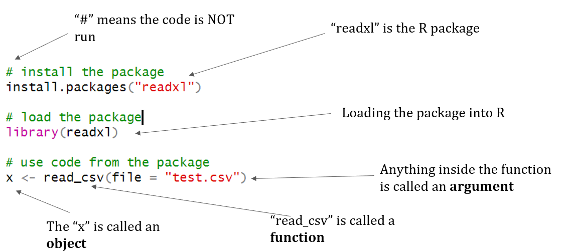
In R, the fundamental unit of shareable code is the package (or library). A package bundles together code, data, documentation, and tests, and is easy to share with others. As of June 2019, there were over 14,000 packages available on the Comprehensive R Archive Network (CRAN), which is the public clearinghouse for R packages. To install a package in R use this code install.packages("package_name").

Common file types associated with R

• .r: An R script
• .rmd: An R markdown file
• .rnw: An R Sweave file
• .rds: A file containing a single R object; can be created by using the function saveRDS() and loaded using the function readRDS()
• .rdata: A file containing one or more R objects or workspaces; can be created using the function save() and loaded using the function load()

Nomenclature of the code

The Data Science Lifecycle

When conducting this tutorial for interns, I like to go step-by-step through the data science lifecycle introduced in the first chapter of R for Data Science by Hadley Wickham and Garrett Grolemund. The introduction details each part of this lifecycle. The first part of this tutorial covers data import and tidying.

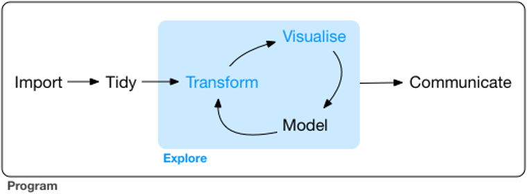
Image courtesy of R for Data Science

File Organization

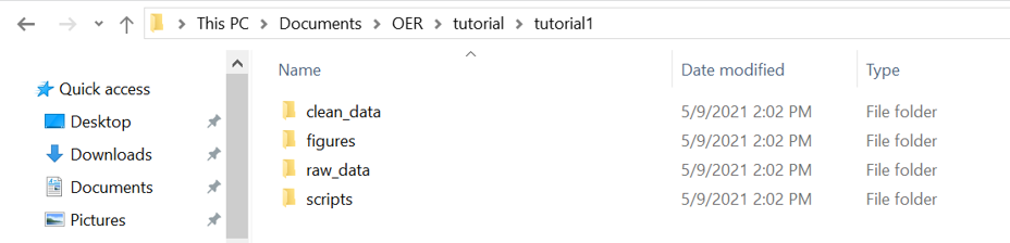
Everyone likes to organize their files differently, but this is the way that I have always done it. I generally have four folders depending on the project I am working on. The "raw_data" folder contains, well, the raw data. This is the data in their rawest format and should not be manipulated or touched at all. I have a folder where I keep all of my R scripts ("scripts"). The "clean_data" folder is any output I generate from my code, whether that be a statistical test in an Excel spreadsheet, intermediate R objects, CSVs, etc. This folder isn't always necessary unless you have multiple scripts that require this intermediate input. Finally, I have a "figures" folder to write out figures for reports or publications.

Introduction to tidyverse

This tutorial exclusively uses packages in tidyverse. The tidyverse is "an opinionated collection of R packages designed for data science. All packages share an underlying design philosophy, grammar, and data structures". The tidyverse packages use the pipe operator, written as %>%. More information about the pipe operator can be found here and in Chapter 18 of R for Data Science. From the article, the pipe operator "takes the output of one function and passes it into another function as an argument. This allows us to link a sequence of analysis steps".

This example is pulled directly from R for Data Science. Here is what the code would look like without the pipe operator:

foo1 <- hop(foo, through = forest)
foo2 <- scoop(foo1, up = field_mice)
foo3 <- bop(foo2, on = head)

And here is what the code would look like using the pipe operator. It allows us to skip those intermediate steps:

clean_foo <- foo %>%
  hop(through = forest) %>%
  scoop(up = field_mice) %>%
  bop(on = head)

Analysis ready data

A dataset is ready for analysis when the data are: quality checked, variables are in columns, and observations are in rows. More information can be found in Chapter 12 of R for Data Science. This image shows an excellent graphical representation of what analysis ready data should look like.

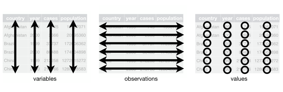
Image courtesy of R for Data Science

Introduction to data analysis and visualization in R

Now that we've covered the basics of R including the importance of cleaning and preparation, it's time to move into data analysis and visulization of the data. At this point, your dataset should be in an analysis ready data format.

Exploratory data analysis

Exploratory data analysis (EDA) is covered in Chapter 7 of R for Data Science. The EDA process can take place throughout the data science lifecycle. EDA is a way to systematically visulize and transform your data in order to further explore them. I tend to explore the data after I have it in the analysis ready data format. There is no right or wrong way to do EDA! This process is an iterative cycle and allows you to:

• Generate questions about your data
• Search for answers by visualizing, transforming, and modeling your data
• Use what you learn to refine your questions and/or generate new questions

Introduction to ggplot2

The package ggplot2 is an R package that comes pre-loaded with the tidyverse. It's used specifically for creating graphs, plots, and other figures. When I need to get started on making a figure I take a look at some of the basic graphs featured in Cookbook for R. This helps me figure out what graph is appropriate for my data and gives me base code to get started on the actual plot.

Statistical tests in R

R comes pre-loaded with a plethora of basic statistical tests. Many packages have improved tests or tests that do not come pre-loaded with R.

• General linear model: lm()
• Generalized linear model: glm()
• ANOVA: anova()
• T-test: t.test()
• Chi-squared test: chisq.test()
• Correlation analysis: cor()
• Summary statistics: mean(), sd(), min(), max(), median()

Ocean exploration data used in this tutorial

The data for this tutorial comes from NOAA's Office of Ocean Exploration and Research (OER or NOAA Ocean Exploration for short). NOAA Ocean Exploration is the only federal program dedicated to exploring our deep ocean, closing the prominent gap in our basic understanding of United States deep waters and seafloor and delivering the ocean information needed to strengthen the economy, health, and security of our nation.

Using the latest tools and technology, NOAA Ocean Exploration explores unknown or poorly known areas of our deep ocean, making discoveries of scientific, economic, and cultural value. Through live video and data streams, online coverage, training opportunities, and events, we allow scientists, resource managers, students, members of the general public, and others to actively experience ocean exploration, allowing broader scientific participation, and cultivating the next generation of ocean explorers, and engaging the public in exploration activities. To better understand our ocean, the office makes exploration data available to the public. This allows us, collectively, to more effectively maintain ocean health, sustainably manage our marine resources, accelerate our national economy, and build a better appreciation of the value and importance of the ocean in our everyday lives.

One way NOAA Ocean Exploration explores is through a dedicated federal ocean exploration vessel called NOAA Ship Okeanos Explorer. Okeanos Explorer is equipped with tools and technologies that allow the office to map and take video and images of the seafloor and water column.

The data from this tutorial come from one of NOAA Ocean Exploration's expeditions called Windows to the Deep 2019, or EX1903. Specifically, the data include two comma separated value (CSV) files of biological and geological observations made during two remotely-operated vehicle (ROV) dives. The data in these CSVs are of the the first two ROV dives of the expedition out of the 19 that were conducted. Each CSV contains annotations that were made of the ROV video data, with each row containing a time stamp of the video with the associated annotation. Scientists and the general public tune into ROV dives live and annotate in real time using SeaTube. For example, if an organism is spotted during the dive, a scientist on shore may timestamp that video and then write in the species identification. Annotations are also quality checked after an expedition. Each annotation also contains associated metadata from the sensors on the ship and the ROV (such as positioning, temperature, salinity, oxygen, depth, etc). All of NOAA Ocean Exploration's data can be accessed through the Digital Atlas portal.

Bubblegum coral, Image courtesy of NOAA Ocean Exploration, Windows to the Deep 2019

R script tutorial

The R script for this tutorial covers most of the data science lifecycle. The first half of the R tutorial script covers installing packages, loading packages, importing files, quality checking the data, and converting the data into an analysis ready format using basic and commonly used functions from the tidyverse packages. The second half uses the analysis ready data to conduct EDA, conduct a statistical test (a t.test specifically), and visualize the data using ggplot2.

Disclaimer

All views expressed on this website are my own and do not represent the opinions of any entity whatsoever with which I have been, am now, or will be affiliated.